
For the love of loops
Loops are control flow statemtents that repeat the same code for a certain number of iterations. So, if you want to do the same thing over and over again, a loop might be exactly what you need. Loops often have a bad reputation among coders because they can be relatively slow and can also be confusing, especially compared to functionals (ex. apply() functions).1 But I can’t deny it, I really love loops. Maybe it’s just how my brain thinks? I find them very intuitive, simple, and effective. I also firmly believe that the best code is the code that does what you want it to do, and makes sense to you (and whoever you need to share it with). So, even if it’s not the most efficient or concise, if your code works for you, then it’s fine code - even if it includes loops. So, let’s talk about loops today. I love loops.
![for (i in 1:4) {person[i] starts walking down the river, away from the camera trap}](../../../posts/2019-09-09-for-the-love-of-loops_files/EK000015.JPG)
for (i in 1:4) {person[i] starts walking down the river, away from the camera trap}
In this post, I want to introduce you to two kinds of loops, and give some simple examples and some more complex ones. This will not be a full comprehensive lesson on loops, but just the stuff that I think is important and fun.
Start by loading the packages we need…
library(tidyverse) #for ggplot2, forcats, purrr, and a few other useful packages
library(sf) #for working with spatial objects
library(adehabitatHR) #for generating spatial objects (note, this includes the pacakge sp)
library(ggspatial) #for adding important map elements (like scales and compasses) to our ggplots
library(viridis) #for pretty colours
library(lubridate) #for dealing with some dates and date-times
Types of loops
There are two kinds of loops (that I know of, at least): “for” loops, and “while” loops. Both types of loops are the same in that they iterate over the enclosed code, over and over again. The main difference between these two types lies basically in what makes them stop iterating:
Forloops repeat code “for the number of iterations that you asked for”Whileloops repeat code “while a certain condition remains true”
Let’s make the simplest example here. I’ll make a for loop that generates 10 random numbers. Then I’ll make a while loop that generates random numbers until it generates a number of 10 or more (then the loop stops). Pay attention to the structure of the loops as well; it’s for or while then the condition in parentheses ( ) and then open wiggly bracket { and put all of the code you want looped after this, and close it with another wiggly bracked }.
set.seed(100)

# the for loop
for (i in 1:10) {                 # condition: i goes from 1 to 10
  my_number <- sample(0:12, 1)    # pick a single random number from 0 to 12
  print(my_number)                # print that number
} # close the wiggly bracket to end the loop
#> [1] 4
#> [1] 3
#> [1] 7
#> [1] 0
#> [1] 6
#> [1] 6
#> [1] 10
#> [1] 4
#> [1] 7
#> [1] 2


# the while loop
my_number <- 0                   # we need to assign a starting value to this variable
while (my_number < 10) {         # condition: my_number is less than 10
  my_number <- sample(0:12, 1)   # pick a single random number from 0 to 12
  print(my_number)               # print that number
} # close the wiggly bracket to end the loop
#> [1] 8
#> [1] 11
So, basically, in both cases, we have a condition (i in 1:10 and my_number < 10) during which the loop should iterate, and then we have an open squiggly bracked { to say “this is what you should do” and a close squiggly bracket } to say “ok, that’s all you need to do, now go back to the start”. Back at the start, the condition is evaluated again, and if satisfied, the code is executed again. Note that for a while loop, any variables in your condition need to already exist, so you should define them before, outside your loop. In a for loop, the variable (i) is automatically assigned to the first value (1) when the loop is started. I think that in while loops, specifying the condition part is probably more intuitive to most people, so I’m going to focus on for loops now…
For loops for me and for you
So, in the case above, the for (i in 1:10) just means “start i at 1, and count it up to 10”. Because we aren’t using the i in that loop, you don’t really get a sense of how that’s working, except you see that after 10 iterations, it ends, so you know that somewhere in the background, i = 1, then i = 2, etc etc, up to i = 10.
One thing that is really nice about for loops is that we can use this built-in loop counter (i.e. the variable i2) to refer to specific input and to organize our output. So let’s try something a little different, where we actually use the i to organize our output…
Simple loops
This time, I want to make a list of ten vectors, each containing 5 random numbers. I’ll start by making my output object, in which to “catch” the random number vectors that I’ll generate. Then, on each iteration of the loop, I’ll have it generate these random numbers, and drop them into the correct “slot” in the list…
((Side note: For these simple loops, I’ll also include the code to use an apply or purrr::map function to achieve the same things. You can decide for yourself which you like best.))
# initiate the list to catch the output
My_random_number_list <- list()


for (i in 1:10) {
  My_random_number_list[[i]] <- sample(1:100, size = 5)  #drop the 5 random numbers into the i'th slot of the list
}

My_random_number_list # take a look at it
#> [[1]]
#> [1] 29 40 75 65 20
#>
#> [[2]]
#> [1]  36 100  68  52  69
#>
#> [[3]]
#> [1] 54 75 42 17 74
#>
#> [[4]]
#> [1] 89 55 28 48 90
#>
#> [[5]]
#> [1] 35 95 69 87 18
#>
#> [[6]]
#> [1] 63 98 13 33 84
#>
#> [[7]]
#> [1] 78 82 60 48 75
#>
#> [[8]]
#> [1] 89 21 31 33 20
#>
#> [[9]]
#> [1] 24 28 58 25 12
#>
#> [[10]]
#> [1] 23 60 21 45 63

# do the same thing with apply and purrr::map, instead of a loop
My_random_number_list_apply <- lapply(X = 1:10,
                                      FUN = function(x) sample(1:100, size = 5))
My_random_number_list_apply
#> [[1]]
#> [1] 97 67 44 35 98
#>
#> [[2]]
#> [1] 45 25 69 40 32
#>
#> [[3]]
#> [1] 58 96 65 61 83
#>
#> [[4]]
#> [1] 78 83  9 45 58
#>
#> [[5]]
#> [1] 92 98  4 57 71
#>
#> [[6]]
#> [1] 25 30 72 88 21
#>
#> [[7]]
#> [1] 36 45 89 38 50
#>
#> [[8]]
#> [1] 13  3 76 32 38
#>
#> [[9]]
#> [1]  5 36 56 67 94
#>
#> [[10]]
#> [1] 71  2 53 82 78

My_random_number_list_map <- map(.x = 1:10,
                                 ~sample(1:100, size = 5))
My_random_number_list_map
#> [[1]]
#> [1]  9 24 95  4 88
#>
#> [[2]]
#> [1] 73 20 83 39 38
#>
#> [[3]]
#> [1] 48 58 35  3 96
#>
#> [[4]]
#> [1] 96 55 10 24 83
#>
#> [[5]]
#> [1] 74 50 57  2 46
#>
#> [[6]]
#> [1]  5 46 62 66  9
#>
#> [[7]]
#> [1] 15 90 13 71 92
#>
#> [[8]]
#> [1]  5  2 20 49 89
#>
#> [[9]]
#> [1] 14 17 60 80 81
#>
#> [[10]]
#> [1] 79  2 69 80 55
And now, let’s use the i to specify our input too. Let’s say that I want to generate an increasing length of random number vector for each list slot. I have another vector already that has ten numbers, each number higher than the previous, and I want the lengths of my random number vectors to correspond to the numbers in this lengths vector….
# this vector has the lengths that i want my random number vectors to each be:
Lengths_of_rndm_number_vecs <- c(5, 17, 21, 30, 42, 51, 66, 74, 89, 91)

# initiate the list to catch the output
My_random_number_list <- list()

for (i in 1:10) {
  My_random_number_list[[i]] <- sample(1:100,         #drop the random numbers into the i'th slot of the list
                                       size = Lengths_of_rndm_number_vecs[i])      #pull the i'th number from the length vector
}

My_random_number_list
#> [[1]]
#> [1] 49 16  9 99  3
#>
#> [[2]]
#>  [1] 71 76 85 43 41 56 78 74 31 88 59 96 54 26 62 79 57
#>
#> [[3]]
#>  [1]  19  35  13  11  29  80  94  41 100  88  60  27  97  53  91  68  32
#> [18]  95  75  67  26
#>
#> [[4]]
#>  [1] 88 80 60  8 41 33 71 21 27 95 57 99 66 40  4 49 37 50 79 22 53  7  6
#> [24] 29 23 42 28 62 45 77
#>
#> [[5]]
#>  [1] 30 38 69 92 75 21 68 62 65 26 97 59  4  6 25 91 81 33 31 98 94 85 11
#> [24] 48 61 79 80 15 58 54 64 23 87 93 70 44 77 28  8 42 90 29
#>
#> [[6]]
#>  [1] 18 67 26 34 21  2 36 53 63 68 86 15 29 12 55 88 90 98  6 54 61 44 43
#> [24] 66 50 72 46 94 71 35 74 42 65 25 58 30 32 91 39 37 48 33 45 24 85 56
#> [47] 81 23 52 41 83
#>
#> [[7]]
#>  [1]  51  91  26  17  39  52  24  35  54  20  73  57  65  96  50  22  87
#> [18]  14 100  78  84  60   2  83  49  13  27  77  88  97  69  81   8  71
#> [35]  48   3  36  44  19  94  63  89  45  34  98  99  21  11  68  55  90
#> [52]  93  82  75  62   9  37  23  67  61  80  56  47  38  59  86
#>
#> [[8]]
#>  [1] 57 51 14 24 69 29 49 26 34 40 73 47 62 74 90 92 13 54 97 76 84 77  1
#> [24] 55 48 58 67 38 83 66  7 35 98 87  3 15 75  8 23 10 11 64 81 79 88 89
#> [47]  4 17 93 33 52 91 28 53 31 60 12 56 46 32  5 82 96 39 61 80 43 30 37
#> [70] 95 44 25  2 70
#>
#> [[9]]
#>  [1] 37 36 28 38 34 27 76 93 70 55 54 52 22 40 86  8  5 41 84 77 51 88 78
#> [24] 98 29 25 85 43 24  1 92 26 15 50 21 95 69 81 48 13 45 35 19 79  2 65
#> [47] 53 71  6 23 16 62 94 59 31 33 82 10 91 87 60 90 64 46 30 99  7  4 68
#> [70] 58 97 75 20 18 42 80 66 63 74 12 32 67 83 49 96 17 57 72  9
#>
#> [[10]]
#>  [1]  24   1  47  85  26  64  83  97  36  79  98  66  93  50  27  95  38
#> [18]  40  39  60   9  51  33  62  90  19  91  96  65  76  89  10  67 100
#> [35]  16  41  48  61  58  49  75   6  13   2  78  80   7   8  88  14  28
#> [52]  32  53  94  74  25  82  87  17  57  15  43  12  30  44  52  77  11
#> [69]  29  34  73  69   4  42  18  54   5  35   3  68  81  71  55  72  20
#> [86]  31  22  23  99  59  70

# do the same thing with purrr::map2, instead of a loop
My_random_number_list_map2 <- map2(.x = 1:10,
                                   .y = Lengths_of_rndm_number_vecs,
                                   ~sample(1:100, size = .y))
My_random_number_list_map2
#> [[1]]
#> [1] 58 32 98 49 66
#>
#> [[2]]
#>  [1] 74 90 44 73 97 43 35  8 19 81 83 55 33 59 36 57 77
#>
#> [[3]]
#>  [1] 42 16 37 46 24 12  1 61  6 95 87 96 94 90 57 62 60 69 13 55 68
#>
#> [[4]]
#>  [1] 100  31  15  51  80  88  33  99  78  41  63  81   3  42  36  29  56
#> [18]  73   8  28  75  83  54  30   1  92  86  76  87   6
#>
#> [[5]]
#>  [1] 38 99 10 79  9 84 93 57 64 46 25  1 59 48 52 27 76 77 80 28 75 73 54
#> [24] 60 91 58  8 17 51  3 45 47 31 95 89  5 18 30 49 23 55 68
#>
#> [[6]]
#>  [1]  29  25  58  37  68  12  57  79  33 100  71  23  74  66  27  39  35
#> [18]  86  95  88  13  67  43   9   4  22  87  62   5  76  89  10   3  77
#> [35]  38  93  49   7  15  28  31  55  96  65  48  94  45  46  84   2  50
#>
#> [[7]]
#>  [1]  15   9  79  34  70  33  81  38  53  83  85  76  37  31  40  77  87
#> [18]  49  52  58   2  86  35  43  14  90  46  47  94  25  24  69  91  28
#> [35]  93   7  56  84  18  29   3  82  44   5  96  61  98 100  26  50  75
#> [52]  89  13  51  67  60  32  72  12  22  95  55  54  80   1  66
#>
#> [[8]]
#>  [1]  25  90  51  68  92   6  13  72  80  67  82  66  15  42  36  40  38
#> [18]   3  54  32  83  23   1  50  63  57  39  46  29  31  45  34  74  35
#> [35]  55  37  78  30  96  88  58  16  62  89  60  81  27  44  28  43   4
#> [52]  65  17  76  69  98  12  87  20  33  49  97   9   8  26  47   2 100
#> [69]  10  85  91  86  19  24
#>
#> [[9]]
#>  [1]  85  96  90  28  44  83  49  25  80  63  54  95  14  71  27  79  55
#> [18]  15  37  62  21 100  41  77  31  99  66  91  76  20  73  69  10  82
#> [35]  92  56   3  24  32  47  18  94   1   2  88  46   4   6  33  35  19
#> [52]   9  57  70  97  75  16   8  42  48  29  78  11  64  61  81  17  36
#> [69]  22  12  30  38  43  84  50  65  51  13  98  74  39  53   7  72  59
#> [86]  52  45  86  93
#>
#> [[10]]
#>  [1]  78  18  77  93  85  90  16  14  97  59  61  60  19  17  42  67  65
#> [18]  44  81  82  43   8  45  11 100  70  15  30  27  54  79   9  49  58
#> [35]  94  83  21  50  41  74  95  62  89  33  76  35  26  34  52  39   7
#> [52]  66  38  56  88  69  84  63  53  29  32  64  99   6  36  20  87  92
#> [69]  47  37  72  46  73  71  25  23  98  28  48  68   3   5  24  75   2
#> [86]  12  13  51  91  57  10
So, in other words, there is a ‘counter’ in the background, represented by i in these cases, and we can use it within the loop itself.
More complicated loops
Now, let’s try something a bit more complicated, using this fake data. (Note: This is not real data. I made it all up.)
In this dataframe, there are 3000 rows, 1000 each for 3 individuals. Each row of data represents an (X, Y) location point, and also includes the Date & Time of that location point.
So let’s say that I want to generate 100 minimum convex polygon home ranges per individual, each one made from 100 randomly selected points (out of the 1000 total). This would be a good job for a for loop…
load("the-right-directory-on-your-computer/loc data.Rdata")# take a look at the data
str(df)
#> 'data.frame': 3000 obs. of 4 variables:
#> $ Focal : Factor w/ 3 levels "OMA","THEO","TOB": 1 1 1 1 1 1 1 1 1 1 ...
#> $ DateTime: POSIXct, format: "2014-08-27 13:00:00" "2014-08-27 13:30:00" ...
#> $ X : num 717 760 761 616 649 ...
#> $ Y : num 1162 1350 1245 1352 1466 ...
ggplot() +
geom_point(data = df,
mapping = aes(x = X, y = Y,
color = Focal),
alpha = 0.5) +
theme_linedraw() +
scale_color_brewer(type = "qual", palette = 2)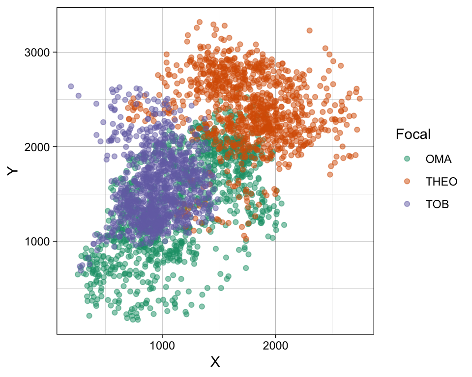
# convert this data to a SpatialPointsDataFrame (so that we can use the mcp function in adehabitatHR)
spdf <- SpatialPointsDataFrame(coords = df[c("X", "Y")],
                               data = df["Focal"])
str(spdf)
#> Formal class 'SpatialPointsDataFrame' [package "sp"] with 5 slots
#>   ..@ data       :'data.frame':  3000 obs. of  1 variable:
#>   .. ..$ Focal: Factor w/ 3 levels "OMA","THEO","TOB": 1 1 1 1 1 1 1 1 1 1 ...
#>   ..@ coords.nrs : num(0)
#>   ..@ coords     : num [1:3000, 1:2] 717 760 761 616 649 ...
#>   .. ..- attr(*, "dimnames")=List of 2
#>   .. .. ..$ : NULL
#>   .. .. ..$ : chr [1:2] "X" "Y"
#>   ..@ bbox       : num [1:2, 1:2] 195 171 2742 3318
#>   .. ..- attr(*, "dimnames")=List of 2
#>   .. .. ..$ : chr [1:2] "X" "Y"
#>   .. .. ..$ : chr [1:2] "min" "max"
#>   ..@ proj4string:Formal class 'CRS' [package "sp"] with 1 slot
#>   .. .. ..@ projargs: chr NA

# split this into a list of spdfs, one per Focal -- this makes it easier to pull out 100 random points
# per focal, in the loop
split_spdf <- split(spdf, spdf$Focal)


# make a list object in which to catch the output
MCP_iterations <- list()

for (i in 1:100) {  # for each of 100 iterations, do the following....

  # pull 100 random rows from each 1000-row spdf in the split_spdf
  split_spdf_sub <- map(split_spdf, ~.x[sample(1:1000, size = 100),])

  # rbind these 3 spdfs in the list back into one single spdf
  spdf_sub <- do.call("rbind", split_spdf_sub)

  # now calculate 95% mcp ranges for that spdf (this function will automatically calculate
  # one mcp per level of the data (in this case "Focal") factor), save it in our output list
  MCP_iterations[[i]] <- mcp(spdf_sub, percent = 95)

  # clean up
  rm(split_spdf_sub, spdf_sub)

} # close up the loop

# take a look at 1 of the outputs
str(MCP_iterations[[1]])
#> Formal class 'SpatialPolygonsDataFrame' [package "sp"] with 5 slots
#>   ..@ data       :'data.frame':  3 obs. of  2 variables:
#>   .. ..$ id  : Factor w/ 3 levels "OMA","THEO","TOB": 1 2 3
#>   .. ..$ area: num [1:3] 213.3 192.1 97.2
#>   ..@ polygons   :List of 3
#>   .. ..$ :Formal class 'Polygons' [package "sp"] with 5 slots
#>   .. .. .. ..@ Polygons :List of 1
#>   .. .. .. .. ..$ :Formal class 'Polygon' [package "sp"] with 5 slots
#>   .. .. .. .. .. .. ..@ labpt  : num [1:2] 1156 1211
#>   .. .. .. .. .. .. ..@ area   : num 2133369
#>   .. .. .. .. .. .. ..@ hole   : logi FALSE
#>   .. .. .. .. .. .. ..@ ringDir: int 1
#>   .. .. .. .. .. .. ..@ coords : num [1:11, 1:2] 1938 1350 894 620 368 ...
#>   .. .. .. .. .. .. .. ..- attr(*, "dimnames")=List of 2
#>   .. .. .. .. .. .. .. .. ..$ : chr [1:11] "99" "83" "66" "75" ...
#>   .. .. .. .. .. .. .. .. ..$ : chr [1:2] "X" "Y"
#>   .. .. .. ..@ plotOrder: int 1
#>   .. .. .. ..@ labpt    : num [1:2] 1156 1211
#>   .. .. .. ..@ ID       : chr "OMA"
#>   .. .. .. ..@ area     : num 2133369
#>   .. ..$ :Formal class 'Polygons' [package "sp"] with 5 slots
#>   .. .. .. ..@ Polygons :List of 1
#>   .. .. .. .. ..$ :Formal class 'Polygon' [package "sp"] with 5 slots
#>   .. .. .. .. .. .. ..@ labpt  : num [1:2] 1818 2426
#>   .. .. .. .. .. .. ..@ area   : num 1921303
#>   .. .. .. .. .. .. ..@ hole   : logi FALSE
#>   .. .. .. .. .. .. ..@ ringDir: int 1
#>   .. .. .. .. .. .. ..@ coords : num [1:12, 1:2] 2640 2650 2119 1738 1363 ...
#>   .. .. .. .. .. .. .. ..- attr(*, "dimnames")=List of 2
#>   .. .. .. .. .. .. .. .. ..$ : chr [1:12] "101" "171" "199" "172" ...
#>   .. .. .. .. .. .. .. .. ..$ : chr [1:2] "X" "Y"
#>   .. .. .. ..@ plotOrder: int 1
#>   .. .. .. ..@ labpt    : num [1:2] 1818 2426
#>   .. .. .. ..@ ID       : chr "THEO"
#>   .. .. .. ..@ area     : num 1921303
#>   .. ..$ :Formal class 'Polygons' [package "sp"] with 5 slots
#>   .. .. .. ..@ Polygons :List of 1
#>   .. .. .. .. ..$ :Formal class 'Polygon' [package "sp"] with 5 slots
#>   .. .. .. .. .. .. ..@ labpt  : num [1:2] 909 1652
#>   .. .. .. .. .. .. ..@ area   : num 972154
#>   .. .. .. .. .. .. ..@ hole   : logi FALSE
#>   .. .. .. .. .. .. ..@ ringDir: int 1
#>   .. .. .. .. .. .. ..@ coords : num [1:9, 1:2] 1387 1238 918 546 508 ...
#>   .. .. .. .. .. .. .. ..- attr(*, "dimnames")=List of 2
#>   .. .. .. .. .. .. .. .. ..$ : chr [1:9] "246" "279" "297" "247" ...
#>   .. .. .. .. .. .. .. .. ..$ : chr [1:2] "X" "Y"
#>   .. .. .. ..@ plotOrder: int 1
#>   .. .. .. ..@ labpt    : num [1:2] 909 1652
#>   .. .. .. ..@ ID       : chr "TOB"
#>   .. .. .. ..@ area     : num 972154
#>   ..@ plotOrder  : int [1:3] 1 2 3
#>   ..@ bbox       : num [1:2, 1:2] 367 292 2650 3279
#>   .. ..- attr(*, "dimnames")=List of 2
#>   .. .. ..$ : chr [1:2] "x" "y"
#>   .. .. ..$ : chr [1:2] "min" "max"
#>   ..@ proj4string:Formal class 'CRS' [package "sp"] with 1 slot
#>   .. .. ..@ projargs: chr NA
So, now I have a list of 100 SpatialPolygonsDataFrames, and each SpatialPolygoneDataFrame has the 95% MCP of each of my 3 animals, using 100 random points each. Let’s say that I’m most interested in the size of their ranges… then I might do something like this…
# create a dataframe of the iteration number, focal IDs, and areas
df_areas <- as.data.frame(cbind(Area = unlist(map(MCP_iterations, `[[`, "area")), #this line PULLS the "area" values out of the SpatPolyDFs
                                Focal = rep(c("OMA", "THEO", "TOB"), times = 100),
                                Iteration = rep(1:100, each = 3)),
                          stringsAsFactors = FALSE)
str(df_areas)
#> 'data.frame':    300 obs. of  3 variables:
#>  $ Area     : chr  "213.336872499984" "192.130308999963" "97.2154224999653" "220.540210499977" ...
#>  $ Focal    : chr  "OMA" "THEO" "TOB" "OMA" ...
#>  $ Iteration: chr  "1" "1" "1" "2" ...
df_areas$Area <- as.numeric(df_areas$Area)

# take a look at it
ggplot() +
  geom_boxplot(data = df_areas,
               mapping = aes(x = Focal, y = Area,
                             color = Focal)) +
  theme_linedraw() +
  scale_color_brewer(type = "qual", palette = 2) +
  theme(legend.position = "none")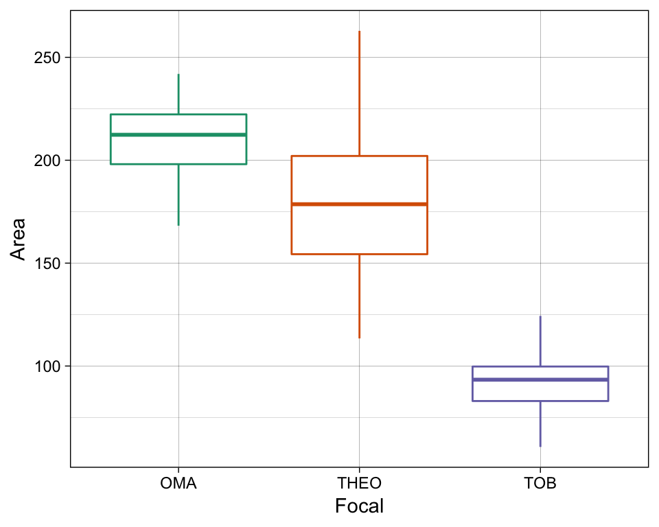
Alright, so now I’d like to a slightly more complicated ’building a new dataframe from another dataset"-style of loop. Along the way, I’ll introduce two useful statements that can be used to alter a normal looping sequence, break and next. The two statements are:
breakis used to basically end the loop completely - so whatever code comes after the loop, and however many more iterations ‘should’ happen, all of that will be skipped if your code gets to abreakstatement.nextis used to skip over whatever code is left within the loop, and go straight to the next iteration.
Generally speaking - and it may already be obvious why - you would embed these statements in an if...else control structure within your loop - so your loop will either end (break) or skip ahead to the next iteration (next) if a certain statement is true.
The following example shows how to loop through the objects in a list and build a new dataframe based on some conditions. I’ll include a ‘counter’ for the output dataframe, so you can see how to very simply uncouple the input iterations (i) from the output positions, incase every single iteration does not produce something for the output. I’m feeling pretty uncreative right now, so this won’t be interesting output…
Basically, I’ll just loop through the MCP_iterations list and build a dataframe with some info, based on certain conditions. For iterations wherin Theo’s range is bigger than Oma’s, I’ll pull the Iteration number and Area of the MCP ranges of Oma and Theo, and where Theo’s range is smaller than Oma’s, I won’t pull any info. I have no idea why I would want to do this, but I think it’s an example in which I can cover a bunch of concepts….
Note: This code is not the most efficient way of acheiving this output, but rather is meant simply to illustrate how to accomplish such a thing.
#initialize the output dataframe
output_df <- data.frame(Focal = character(),
                        Iteration = numeric(),
                        Area = numeric(),
                        stringsAsFactors = FALSE)

output_row_number <- 1 #start a counter for the output rows

for (i in 1:length(MCP_iterations)) {


  if (MCP_iterations[[i]]$area[2] < MCP_iterations[[i]]$area[1]) {
  #if Theo's mcp (in slot 2) is smaller than Oma's (in slot 1), then...
    next #skip ahead to the next iteration (the next value of i)
  }

  #otherwise... (i.e. if the next statement wasn't triggered, this code will run...)

  #dump the name Oma into the focal column of the current output_row number
  output_df[output_row_number, "Focal"] <- "Oma"

  #dump the iteration number (which is i, since we're looping through the MCP_iteration list)
  #into the Iteration column of the current output_row_number
  output_df[output_row_number, "Iteration"] <- i

  #pull the first area size (slot 1 is always Oma) and dump it into the Area column
  # of the current output_row_number
  output_df[output_row_number, "Area"] <- MCP_iterations[[i]]$area[1]

  #Now do all the same for Theo, but instead of dumping it into the
  #current output_row_number, dump it into the next one (ie. output_row_number + 1)

  output_df[output_row_number + 1, "Focal"] <- "Theo"
  output_df[output_row_number + 1, "Iteration"] <- i
  output_df[output_row_number + 1, "Area"] <- MCP_iterations[[i]]$area[2]

  #Now add 2 to the current output_row_number, so that the next time we go around,
  #the next data will go AFTER what we just put in
  output_row_number <- output_row_number + 2

}

#take a look at the output
output_df
#>    Focal Iteration     Area
#> 1    Oma         7 175.0242
#> 2   Theo         7 193.9058
#> 3    Oma        11 230.1670
#> 4   Theo        11 262.8734
#> 5    Oma        12 191.3407
#> 6   Theo        12 246.2197
#> 7    Oma        19 197.9443
#> 8   Theo        19 254.9434
#> 9    Oma        26 220.3774
#> 10  Theo        26 233.1131
#> 11   Oma        30 173.5678
#> 12  Theo        30 174.5970
#> 13   Oma        34 215.5322
#> 14  Theo        34 228.4803
#> 15   Oma        41 226.1519
#> 16  Theo        41 259.4007
#> 17   Oma        44 205.9984
#> 18  Theo        44 229.1138
#> 19   Oma        50 186.0953
#> 20  Theo        50 203.6450
#> 21   Oma        53 214.1360
#> 22  Theo        53 228.9846
#> 23   Oma        56 168.1853
#> 24  Theo        56 203.6287
#> 25   Oma        59 209.6801
#> 26  Theo        59 227.0665
#> 27   Oma        65 212.6788
#> 28  Theo        65 215.5359
#> 29   Oma        72 213.2865
#> 30  Theo        72 216.1962
#> 31   Oma        78 207.7069
#> 32  Theo        78 230.4460
#> 33   Oma        79 192.8508
#> 34  Theo        79 196.2322
#> 35   Oma        83 195.4658
#> 36  Theo        83 213.4525
#> 37   Oma        89 205.0556
#> 38  Theo        89 207.2991
#> 39   Oma        95 175.6461
#> 40  Theo        95 183.3611
So, in the above example, you can see how a next statement can be incorporated, and how to use a counter for your output, when you know that each iteration of input won’t produce one row/object of output.
One last little thing
A common mistake that people make in their loops is ‘rebuilding’ each output object in every iteration. Consider these next two simple examples, which each accomplish the same task of constructing a vector of 5 random numbers between 1 and 10:
# Version 1
output_1 <- vector()

for (i in 1:5) {
  output_1 <- c(output_1, sample(1:10, 1))
}

# Version 2
output_2 <- vector()

for (i in 1:5) {
  output_2[i] <- sample(1:10, 1)
}
So in “Version 1”, the output_1 <- c(output_1, sample(1:10, 1)) line of code essentially rebuilds output_1 by taking whatever is already there for output_1, and attaching another random number to the end of it. So, essentially, it is rebuilding the output_1 object in every iteration. Whereas in “Version 2”, the output_2[i] <- sample(1:10, 1) line of code indexs into output_2 using [ ] and says specifically which position (i) the random number should be dumped into. With this simple loop, it makes no difference (except, try rerunning both loops without first removing the output_1 and output_2 objects from your workspace and see what happens…) which you use. But if you were, for example, running a more complicated loop that was building a larger dataframe or some such object, you would really notice the difference in the time it takes to compute the loop using these two different ways of ‘building’ your output objects.
Concluding thoughts
I love loops. There is so much more that I want to put in this post, but I think I’ll save it for another day…. so stay tuned for more about while loops, and embedding loops in loops, and more. For now though, just go have some fun playing around with loops. If you want to know more, I recommend the chapter about “Iteration” in R for Data Science by Hadley Wickham and Garrett Grolemund. Actually, I just recommend this entire book. Enjoy!
Footnotes
From what I’ve read, most of the criticism of loops come from the fact that loops are slow (which is not necessarily true), not very transparent (what is actually going in and what is actually coming out - especially in the case of longer, nested loops with
ifandelsecontrol structures, etc - is not always very clear without doing some digging), and they are commonly used in situation where a functional (ex.applyorpurrr::map) would work just as well (and be at least cleaner, if not faster). While these are valid criticisms, again remember that the best code is the code that does what you want it to do, and that you can understand. So, if that means using a loop that may be slightly less efficient (in terms of time and lines of code), so be it. That said, for a nice introduction to functionals (though, note that this is generally more advanced stuff), check out the Functonals chapter in Advanced R.↩The use of
ifor this variable is basically totally arbitrary. We could also usejorshoesor literally anything. As far as I can tell (from the briefest of google searches), “i” is usually used simple because it stands for “iteration”. If you’re going to be sharing your code with other people, it’s nice to stick to these types of coding norms, because it makes your code more comprehendable to others. If your code is just for you though, then use whatever you want.↩